A Beginner's Guide to Recurrent Neural Networks (Part 2 of 2)

Hi, I am Japkeerat. I am working as a Machine Learning Engineer since January 2020, straight out of college. During this period, I've worked on extremely challenging projects - Security Vulnerability Detection using Graph Neural Networks, User Segmentation for better click through rate of notifications, and MLOps Infrastructure development for startups, to name a few. I keep my articles precise, maximum of 4 minutes of reading time. I'm currently actively writing 2 series - one for beginners in Machine Learning and another related to more advance concepts. The newsletter, if you subscribe to, will send 1 article every Thursday on the advance concepts.
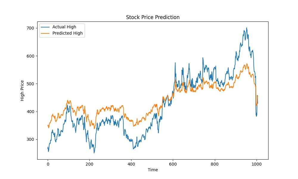
By the end of this tutorial, you’ll have this.

Let’s get started.
For the purpose of this tutorial, I am using Netflix Stock Price Data available on Kaggle and only choose to predict the Daily High of the stock price.
Step 1 - Preprocess the Data
from sklearn.preprocessing import MinMaxScaler

high_data = data["High"].values.reshape(-1,1)

scaler = MinMaxScaler()
scaled_high_data = scaler.fit_transform(high_data)
The code snippet above does 2 things.
First, it selects only the “High” column data and converts it into a NumPy Array. Then it changes its shape. Understand this from the example.
data["High"].values
This part of the code is responsible for converting the “High” column data to a NumPy Array. It will give the output like
[10,20,30,40,50]
Then, .reshape(-1,1) converts this array into a two-dimensional array where in each dimension, you have only 1 element. The output of the above array now looks like this
[[10],
 [20],
 [30],
 [40],
 [50]]
Step 2 - Preparing the Dataset
def create_dataset(dataset, time_step=1):
    X, Y = [], []
    for i in range(len(dataset)-time_step-1):
        a = dataset[i:(i+time_step), 0]
        X.append(a)
        Y.append(dataset[i + time_step, 0])
    return np.array(X), np.array(Y)


X, y = create_dataset(scaled_high_data)

X = X.reshape(X.shape[0], X.shape[1], 1)
In Step 2 of this tutorial, we're preparing our dataset for the RNN model.
The `create_dataset` function is key here. It takes our scaled stock price data and creates sequences for training. Each sequence consists of consecutive days' 'High' prices, determined by time_step. If `time_step` is 1, we use today's price to predict tomorrow's. The function goes through the entire dataset, creating these sequences (X) and their next day's price (Y). Finally, we reshape X to fit the RNN's expected input shape, making it ready for the neural network to process.
This step is crucial as it aligns our data with the way RNNs learn temporal patterns.
Step 3 - Keras Model
model = Sequential()

model.add(SimpleRNN(units=50, activation="relu", input_shape=(1,1)))
model.add(Dense(units=1))

model.compile(optimizer="adam", loss="mean_squared_error")

model.fit(X, y, epochs=2, batch_size=16, verbose=1)
The process of developing a model with Keras begins by initializing a Sequential model, which allows us to stack layers linearly. Within this model, we add a SimpleRNN layer with 50 units. The activation function 'relu' helps the model learn non-linear patterns. The input_shape is set according to our preprocessed data. Next, we add a Dense layer with a single unit. This is our output layer that will predict the next day's 'High' value.
The model is compiled with the 'adam' optimizer and 'mean_squared_error' loss function, both standard choices for regression problems. Finally, we fit the model to our prepared data (X and y). The epochs parameter controls how many times the model will see the entire dataset, and batch_size determines how many data points the model sees before updating its internal parameters. With these steps, our model is ready to learn from the data and make predictions.
And that’s it, you are ready to run the code and build your own Stock Price Prediction Model.


